Traceability of Bulk Materials

Traceability generally describes the ability to track a product throughout its life cycle and assign all relrevant information to itself. This system has largely become a standard for piece goods, whereby e.g. a system of labelling and scanning along the supply chain is implemented. Due to that, all relevant information of each individual prodcut can be saved and called up at any time. This system is particularly widespread in the food industry due to legal regulations (in the EU). Nowadays it is possible to get nearby all relevant information about a food product using the barcode.
“The traceability of food, feed, food-producing animals, and any other substance intended to be, or expected to be, incorporated into a food or feed shall be established at all stages of production, processing and distribution. Food and feed business operators shall be able to identify any person from whom they have been supplied with a food, a feed, a food-producing animal, or any substance intended to be, or expected to be, incorporated into a food or feed. […] Food and feed business operators shall have in place systems and procedures to identify the other businesses to which their products have been supplied. This information shall be made available to the competent authorities on demand. […]”
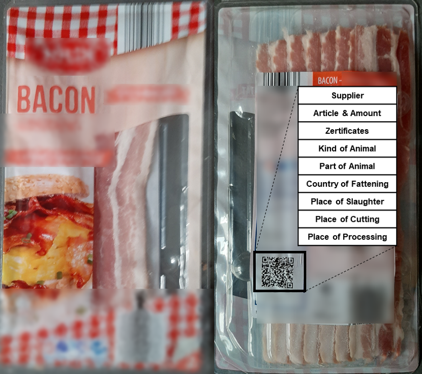
An example of food traceability is the packaging of a BACON (Figure 1). The barcode provides all important informations about the meat. These informations include the country of fattening as well as place of slaughter. Furthermore, the label can provide informations about the further processing and the quality monitoring.
Considering the previous process chain, the following question arises: To what extent can the quality of the animal feed be ensured? It is obvious that marking every single grain is not an option. Hence, a closer look at the traceability of bulk materials at all is essential. The following section shows a typical process chain on the example: from grain to feed. This example can be also applied to any other process chain in which bulk materials are stored and handled.
In practice two major problems occur when considering the traceability of bulk materials: First, a long time can pass between the delivery and the detection of the contamination during discharge of the grain from the silo. Second, the content inside the silo is mixed all the time during the discharge. Hence a trivial classification like FIFO – First In First Out – is not easy to mention. The flow behaviour of the bulk material has to be considered. Obviously, a simple measurement of the filling level of the silo will also give no information about the cereal belonging to a farmer.
The following example shows a typical, simplified process chain. Three different farmers each supply a silo (A and B) at level I. Additional trucks transport the cereals from the two silos (A and B) and deliver them to a common third silo (C) at level II. Thus, Silo A contains cereals from farmers 1, 2, 3 and Silo B cereals from farmers 4, 5, 6. In the silo C there are cereals from all the farmers.
If contamination is found when removing from silo C, the question of traceability arises. In other words, is it possible to assign the bulk material to a silo of the preliminary stage? Or even to a farmer on the first level? To further simplify this problem, we first consider only the beginning of the upper process chain: from farmers 1, 2, 3 and silo A to the transporter. Here the major challenge considering the flow behaviour inside the silo will be presented in general.
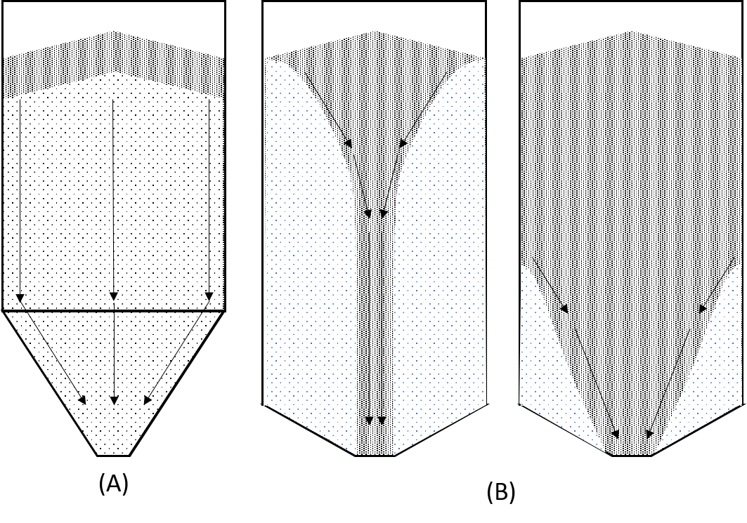
The main problem of tracking the cereals inside the silos results from the flow behaviour during the discharge. From the point of view of an even discharge of the silo, mass flow silos (Figure 3.A) would be preferable. The bulk material flows down almost uniformly in mass flow silo. In practice, however, core flow silos (Figure 3.B) are more common because they allow a higher storage capacity. In contrast to mass flow silos, the material in core flow silos does not flow to the outlet in horizontal layers. Rather, the material flows in the middle first. As a result of progressive discharge, the silo content is mixed. Hence, a “First In – First Out” classfication is not valid in core flow silos.
For a better understanding we consider again the filling and emptying of the silo A of the previous example. The silo is supplied by three farmers with cereals and one truck discharges the cereals from the silo. For each truck load, the operator of the silo wants to determine which farmer the cereals belong to.
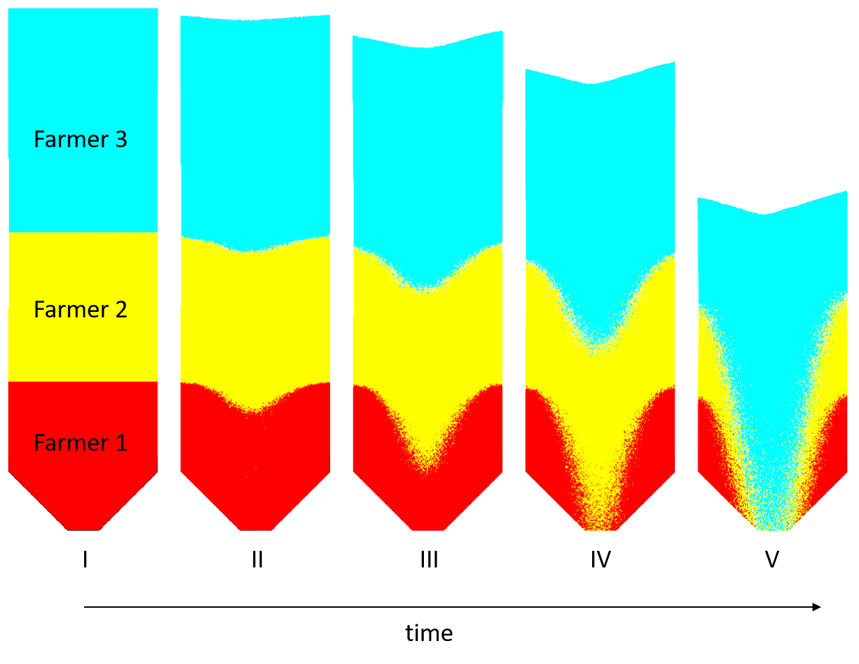
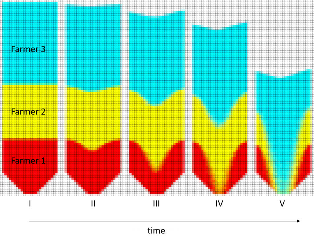
Figure 4 shows the filling status of the core flow silo A at different times. This silo has been simulated by Discrete Element Method (DEM). In general, the layers of bulk material flow unevenly over time and mix like previously explained. At the beginning, an ideal filling is assumed. Each layer can be assigned to one of the three farmers. Now the trucks start emptying the silo. Up to a filling level III, the cereals in the trucks comes exclusively from the first farmer. The beginning of mixing of the layer has no influence yet.
At stage IV the cereal layer of farmer 2 reaches the outlet of the silo. From now on the truck loads include cereals from farmer 1 and farmer 2, but no cereals from farmer 3. Furthermore, the proportion of cereals from farmer 2 increases and that from farmer 1 decreases. At the last stage V also the layer of farmer 3 reaches the outlet of the silo. It should be noted that at this point in time, silo A still contains cereals from farmers 1 and 2. Hence, from now on the truck loads include cereals from farmer 1, farmer 2 and farmer 3. A closer look at the colours of the layers at the outlet shows that the blue layer (farmer 3) dominates. This means that the percentage of cereals from farmer 3 is the largest. This proportion will increase with further discharging.
According to the example, it should be possible to make a statement about every truck load in reality. On the one hand, certain farmers can be excluded. On the other hand, the cargo can be assigned to specific farmers. Furthermore, it should be possible to say what percentage of the truck load belongs to a particular farmer.
This section provides a brief overview of possible solutions for the traceability of bulk materials. Basically, technical sensors are available on the one hand and simulation methods on the other. The individual solutions are briefly outlined and their advantages and disadvantages for practical use are explained.
When considering technical sensors, permanently installed sensors in the silo are excluded. These sensors can only provide information about the general filling state of the silo. When considering segregation of the individual layers within the silo, they cannot provide any further information. Instead, sensors are required that can be inserted directly into the bulk material during the filling. Hence, these sensors are distributed over the entire bulk material, so that there are several sensors in each layer. When emptying these sensors flow with the bulk material. A suitable sensor for this application is the RFID transponder.
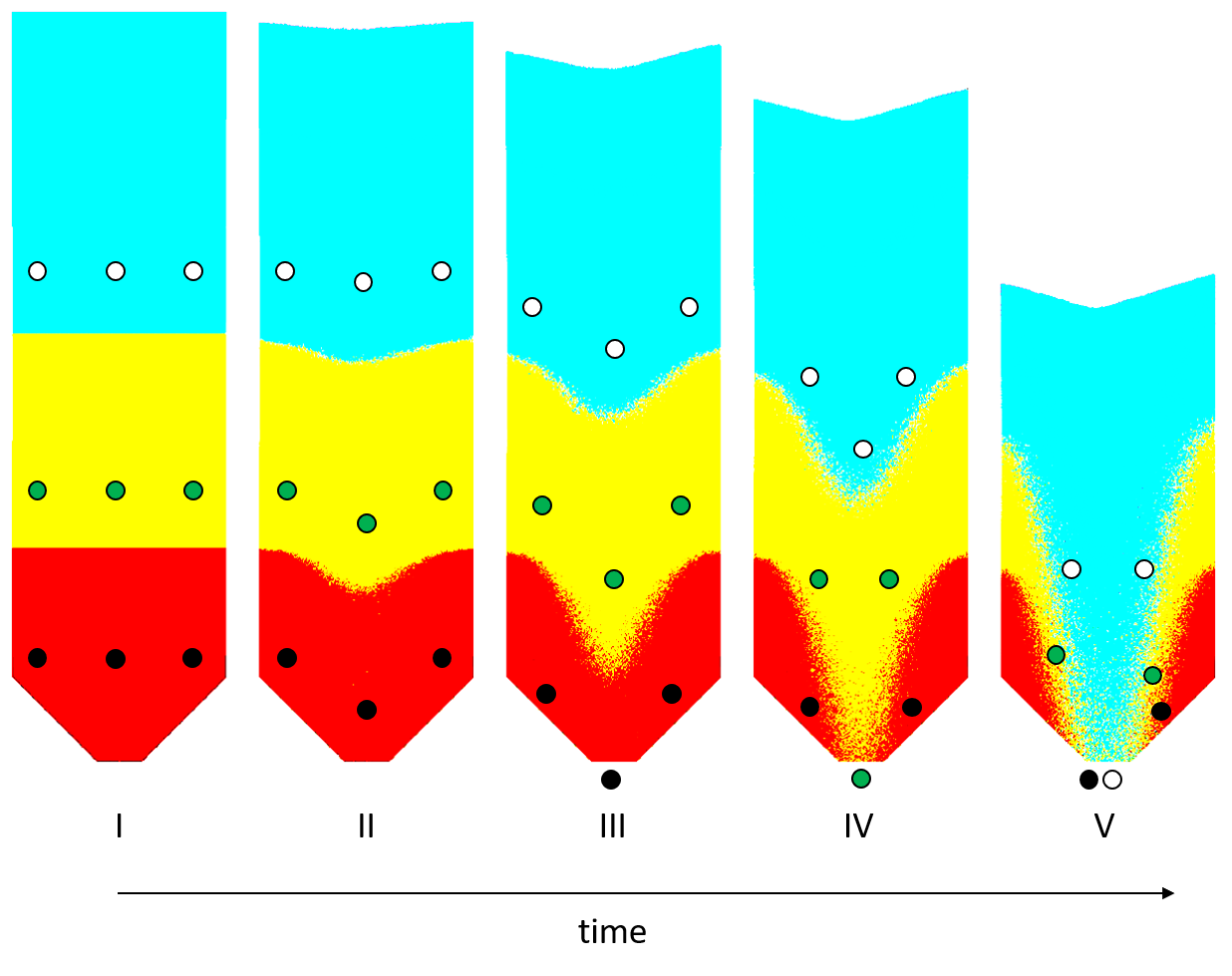
Figure 5 shows the filling of the silo A over time from the previous example. In each layer RFID transponders have been placed. At the outlet a gate way detects the RFID transponder, when it is discharged.
Even if it is known that the cereals at the beginning belong to farmer 1, we will not get any information until point III. At this point the first RFID transponder is recognized.
A similar problem exists at point IV. Here, the first transponder of farmer 2 leaves the silo. However, the operator has no information about how much material from farmer 2 has flowed out before the detection of the transponder. In addition, he does not receive any information if the cereal layer of farmer 1 is still flowing or not. The remaining transponders of farmer 1 are still in the silo.
A more precise resolution can certainly be achieved with additional transponders. However, this also means higher investment costs and additional handling effort. The operator must ensure that all transponders after discharge are removed from the bulk material. Furthermore, the RFID transponder may not flow with its layer and a traceability of the segregation would be not possible.
The previous Figures have been created by simulating a real silo discharge. In general, computer simulations based on the Discrete Element Method (DEM) offer very detailed and physically based options to model the flow of individual particles in the silo or in the stockpile. Therefore, the DEM offers the greatest level of detail for the traceability of bulk materials within a silo simulation. A disadvantage, however, is the high number of particles required for the real representation of a silo. This results in a enormous computing time ranging from a few days to weeks. Even a simplified representation using less number of particles, the computing time is still too long. Therefore, real-time traceability is not possible with this method. For further details about DEM click here.
The cellular automaton is a purely stochastic simulation. Compared to the DEM, the cells in a cellular automaton are only moved according to relative probabilities. No physical interactions are calculated during the simulation. In order to map the same flow behavior anyway, boundary conditions for the probabilities of each individual cell are calibrated. These boundary conditions depend on the real bulk material and the state of the neighboring cells. Therefore, it is necessary to set the probabilities for the cells in such a way that the flow behavior corresponds very well to physical models and reality. Once the probability rules have been set, no adjustment is necessary during the simulation.
The major advantage of the cellular automaton is its simplicity. A correctly calibrated cellular automat shows the same discharge and filling properties as the real system. At the same time, only a fraction of the computing time is necessary to achieve the same quality of the state representation as with the DEM simulation. Hence, it is possible to simulate the filling and discharge of silo capacity of 10,000 m³ with an accuray of 1 liter in realtime using a personal computer. For further information about cellular automaton and silo management click here.
We use cookies on our website. Some of them are essential, while others help us to improve this website and your experience.
Here you will find an overview of all cookies used. You can give your consent to whole categories or display further information and select certain cookies.
Essential cookies enable basic functions and are necessary for the proper function of the website.
| Name | |
|---|---|
| Provider | Owner of this website |
| Purpose | Saves the visitors preferences selected in the Cookie Box of Borlabs Cookie. |
| Cookie Name | borlabs-cookie |
| Cookie Expiry | 1 Year |
Marketing cookies are used by third-party advertisers or publishers to display personalized ads. They do this by tracking visitors across websites.
| Accept | |
|---|---|
| Name | |
| Provider | Google LLC |
| Purpose | Cookie by Google used for website analytics. Generates statistical data on how the visitor uses the website. |
| Privacy Policy | https://policies.google.com/privacy?hl=en |
| Host(s) | |
| Cookie Name | _ga,_gat,_gid |
| Cookie Expiry | 2 Years |
Content from video platforms and social media platforms is blocked by default. If External Media cookies are accepted, access to those contents no longer requires manual consent.
| Accept | |
|---|---|
| Name | |
| Provider | YouTube |
| Purpose | Used to unblock YouTube content. |
| Privacy Policy | https://policies.google.com/privacy?hl=en&gl=en |
| Host(s) | google.com |
| Cookie Name | NID |
| Cookie Expiry | 6 Month |